Advanced Friction
This tutorial describes three advanced friction features:
See also
For an introduction to friction modeling and the dissipative potential, see “Getting Started”.
Spatially Varying Coefficients of Friction
Deprecated
Spatially varying coefficient of friction is achieved by assigning coefficients to each vertex in the mesh. However, friction coefficients are not a material property and should instead be assigned to the contact pair. This feature will be replaced with a per-pair friction coefficient in a future release.
You can specify spatially varying coefficients of friction by passing an Eigen::VectorXd to TangentialCollisions::build. Each entry is the coefficient of friction for one vertex. You can assign different coefficients to different parts of the mesh (e.g. rubber in one region, plastic in another).
You can also provide an optional blend_mu parameter to blend the coefficient of friction on either side of the contact. The default behavior is to average the coefficients of friction on both sides, but you can specify a custom blending function if needed (e.g., multiplying them or taking the maximum or minimum).
Separate Coefficients for Static and Kinetic Friction
Experimental Feature
The support for separate static and kinetic friction coefficients is an experimental feature introduced in v1.4.0. The behavior may be improved in future releases.
Traditionally, friction is modeled with a single coefficient. However, physical systems often exhibit different resistance to motion when at rest (static friction) versus when sliding (kinetic friction). The IPC Toolkit supports specifying both:
Static friction coefficient (
mu_s): Governs the maximum force resisting the initiation of motion.Kinetic friction coefficient (
mu_k): Governs the force resisting ongoing motion.
Usage
To use separate static and kinetic friction coefficients, you can pass them as parameters when building the tangential collisions:
ipc::BarrierPotential B(dhat, barrier_stiffness);
ipc::TangentialCollisions tangential_collisions;
tangential_collisions.build(
    collision_mesh, vertices, collisions, B, mu_s, mu_k);
B = ipctk.BarrierPotential(dhat, barrier_stiffness)
tangential_collisions = ipctk.TangentialCollisions()
tangential_collisions.build(
    collision_mesh, vertices, collisions, B, mu_s, mu_k)
How It Works
Background
IPC defines the local friction force as
where \(\lambda\) is the contact force magnitude, \(T(x) \in \mathbb{R}^{3 n \times 2}\) is the oriented sliding basis, and \(\mu\) is the local friction coefficient. The function \(f_1\) is a mollifier that smooths the transition between static and kinetic friction defined as
where \(\epsilon_v\) is a small constant (e.g., 0.001). The following plot shows the behavior of the function \(f_1\):
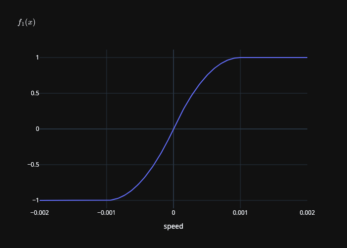
Smooth mollifier \(f_1(\|\mathbf{u}\|)\) where \(\epsilon_v = 0.001\).
To create a dissipative potential we integrate \(f_1\) to obtain a smooth mollifier \(f_0\):
The following plot shows the behavior of the function \(f_0\):
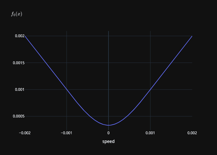
Integrated mollifier \(f_0(\|\mathbf{u}\|)\) where \(\epsilon_v = 0.001\).
Smooth \(\mu\)
When adding separate coefficients for static and kinetic friction, we need to maintain the \(C^1\) continuity of the friction force. This leads us to define a smooth coefficient of friction \(\mu(y)\) that transitions between the static and kinetic coefficients based on the magnitude of the relative velocity \(y = \|\mathbf{u}\|\). The smooth coefficient of friction is defined as
We plot the smooth coefficient of friction \(\mu(y)\) below:
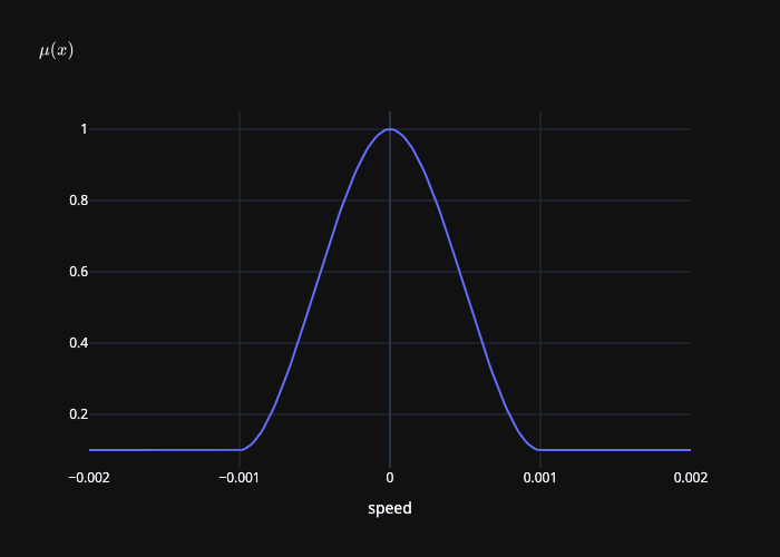
Smooth coefficient of friction \(\mu(\|\mathbf{u}\|)\) where \(\mu_s = 1\), \(\mu_k = 0.1\), and \(\epsilon_v = 0.001\).
Smooth \(\mu\) Mollifier
Using a smooth function \(\mu(\|\mathbf{u}\|)\) instead of a constant \(\mu\) gives a smooth transition between static and kinetic friction. The function \(\mu(\|\mathbf{u}\|) f_1(\|\mathbf{u}\|)\) is plotted below:
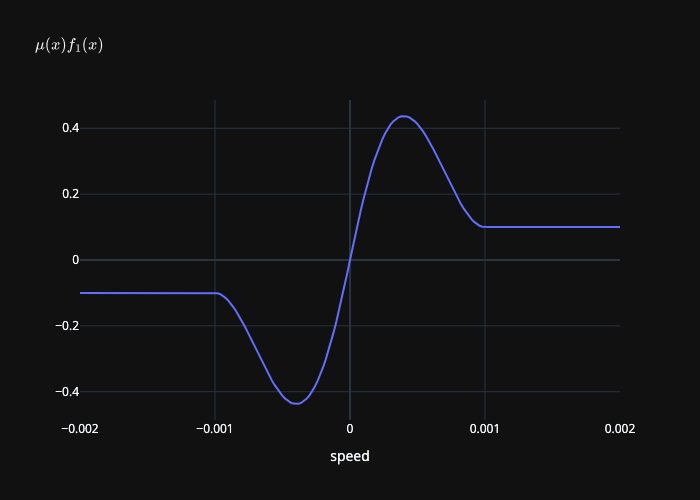
Smooth coefficient of friction multiplied by the friction mollifier \(\mu(\|\mathbf{u}\|) f_1(\|\mathbf{u}\|)\) where \(\mu_s = 1\), \(\mu_k = 0.1\), and \(\epsilon_v = 0.001\).
However, \(\frac{\mathrm{d}}{\mathrm{d}y} \mu(y) f_0(y) \neq \mu(y) f_1(y)\), so we need to adjust the integrated mollifier by integrating the product of the smooth coefficient of friction and the mollifier:
The following plot shows the behavior of the integrated mollifier multiplied by the smooth coefficient of friction:
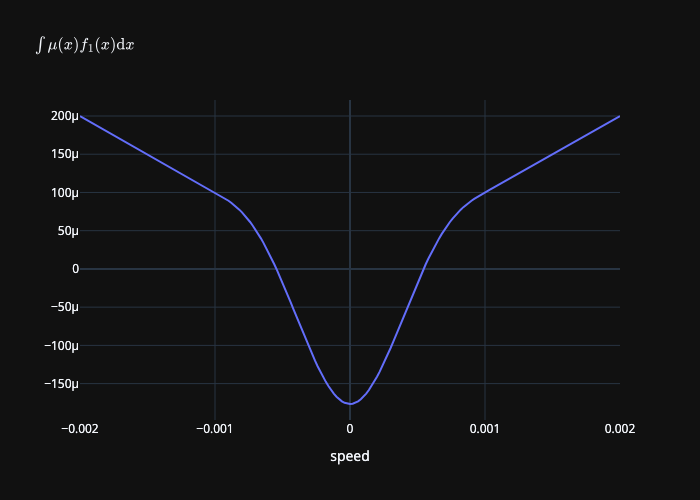
Integrated mollifier \(\int \mu(y) f_1(y) \mathrm{d} y\) where \(\mu_s = 1\), \(\mu_k = 0.1\), and \(\epsilon_v = 0.001\).
Discussion
While this approach provides a smooth transition between static and kinetic friction, there are some considerations:
- The product \(\mu(y) f_1(y)\) underestimates the friction force in the static regime, which may lead to less accurate simulations of static friction.
This is, when \(\mu_k < \mu_s\) and \(|y| \leq \epsilon_v\), \(\max(\mu(y) f_1(y)) < \mu_s\).
We could address this by scaling by \(\frac{\max(\mu(y) f_1(y))}{\mu_s}\), but computing the maximum is non-trivial.
- The combined function \(\mu(y) f_1(y)\) is a degree 4 polynomial, which is more complex than the original mollifier \(f_1(y)\) (degree 2). This may lead to more difficult to optimize problems.
We could replace \(\mu(y) f_1(y)\) with a piecewise quadratic function that has the desired behavior. This help with (1) as well. However making it backwards compatible with the original mollifier is challenging.
If you have suggestions for improving this approach or alternative methods, please reach out on our GitHub Discussions.
Anisotropic Friction
See also
C++ API and Python API for the anisotropic
helpers. The notebooks/anisotropic_friction_math.ipynb notebook has the
full derivation and plots.
New Feature
Anisotropic friction uses direction-dependent coefficients (e.g. wood grain, brushed surfaces).
You can set different friction coefficients along each tangent direction. Wood (along vs. across the grain) and brushed metal are typical cases.
Directions tangent to the mesh
The two anisotropy axes are the contact’s tangent basis. They lie in the
plane tangent to the contact and are computed from the collision geometry.
You do not pass a custom 3D direction (e.g. a world-space “grain” vector).
You pass coefficients only: mu_s_aniso and mu_k_aniso are 2D vectors
whose first component is along the first tangent direction and second along
the second. So anisotropy is always along the mesh tangent directions at
each contact.
Setting coefficients (component 0 = first tangent direction, component 1 = second, both tangent to the surface):
for (size_t i = 0; i < tangential_collisions.size(); ++i) {
    // Component 0 = first tangent dir, 1 = second (tangent to surface)
    tangential_collisions[i].mu_s_aniso = Eigen::Vector2d(0.8, 0.4);
    tangential_collisions[i].mu_k_aniso = Eigen::Vector2d(0.6, 0.3);
}
for i in range(len(tangential_collisions)):
    # Component 0 = first tangent dir, 1 = second (tangent to surface)
    tangential_collisions[i].mu_s_aniso = np.array([0.8, 0.4])
    tangential_collisions[i].mu_k_aniso = np.array([0.6, 0.3])
Anisotropic friction uses an elliptical \(L^2\) projection model. For a given tangential velocity direction \(\mathbf{t} = \boldsymbol{\tau} / \|\boldsymbol{\tau}\|\), the effective friction coefficient is:
where \(\mu_0\) and \(\mu_1\) are the friction coefficients along the two tangent basis directions, and \(t_0\) and \(t_1\) are the components of the unit direction vector. This formulation matches the matchstick (elliptical Coulomb cone) model. See Erleben et al. [2019].
Usage
To use anisotropic friction, you can assign anisotropic friction coefficients to each tangential collision after building the collisions:
ipc::BarrierPotential B(dhat, barrier_stiffness);
ipc::TangentialCollisions tangential_collisions;
tangential_collisions.build(
    collision_mesh, vertices, collisions, B, mu_s, mu_k);

// Assign anisotropic friction coefficients per collision
for (size_t i = 0; i < tangential_collisions.size(); ++i) {
    // Components 0 and 1 = contact's two tangent dirs (tangent to surface)
    tangential_collisions[i].mu_s_aniso = Eigen::Vector2d(0.8, 0.4);
    tangential_collisions[i].mu_k_aniso = Eigen::Vector2d(0.6, 0.3);
}

// Refresh lagged matchstick μ from lagged geometry and slip (e.g. each Newton iteration)
tangential_collisions.update_lagged_anisotropic_friction_coefficients(
    collision_mesh, rest_positions, lagged_displacements, velocities);
B = ipctk.BarrierPotential(dhat, barrier_stiffness)
tangential_collisions = ipctk.TangentialCollisions()
tangential_collisions.build(
    collision_mesh, vertices, collisions, B, mu_s, mu_k)

# Assign anisotropic friction coefficients per collision
for i in range(len(tangential_collisions)):
    # Components 0 and 1 = contact's two tangent dirs (tangent to surface)
    tangential_collisions[i].mu_s_aniso = np.array([0.8, 0.4])
    tangential_collisions[i].mu_k_aniso = np.array([0.6, 0.3])

tangential_collisions.update_lagged_anisotropic_friction_coefficients(
    collision_mesh, rest_positions, lagged_displacements, velocities)
Lagged effective μ (direction-dependent coefficients)
When mu_s_aniso / mu_k_aniso are nonzero, the toolkit lags the
matchstick effective coefficients for the current nonlinear step (stored in
mu_s_effective_lagged and mu_k_effective_lagged on each
TangentialCollision). Call
TangentialCollisions::update_lagged_anisotropic_friction_coefficients with
rest positions, lagged displacements, and velocities whenever those change
(e.g. each Newton iteration), after assigning per-collision ellipse axes. This
is analogous to lagging the tangent frame and normal data in IPC, and it
keeps the friction dissipative potential consistent with the friction force for
that step (a path-dependent μ that updates every iteration would not admit an
exact incremental potential).
Friction Jacobians in the toolkit omit \(\partial \mu / \partial \tau\) for
this direction-dependent case because \(\mu_{\text{eff}}\) is held fixed
after the lag update.
Directional lagged-\(\mu\) refresh is currently activated when
mu_s_aniso is nonzero in a 2D tangent space. If only
mu_k_aniso is nonzero, the current gate keeps isotropic lagged
coefficients.
For discussion of the curl / non-conservative-field issue and the lagged-μ
recommendation in IPC, see the maintainer notes linked from
PR #210 (and
Erleben et al. [2019] for the matchstick cone).
Relationship with Other Anisotropy Mechanisms
Two mechanisms are available:
Velocity scaling (
mu_aniso): component-wise scaling of the tangential velocity before friction; changes the effective speed in the friction law.Ellipse coefficients (
mu_s_aniso,mu_k_aniso): different \(\mu\) along each tangent direction.
Use one or both. When both are set, velocity scaling is applied first; the
ellipse effective \(\mu\) is then chosen from the direction of that scaled
slip when you call update_lagged_anisotropic_friction_coefficients.
Future Directions
Planned or under discussion: velocity-dependent friction and rolling friction. See the project’s GitHub for current status or to contribute.